Template

New!

We just launched a new >30 hour video course for more experienced students:

Practical Deep Learning for Coders part 2: Deep Learning Foundations to Stable Diffusion

Data Storage

Data sourcing and data storage go hand-in-hand and it is necessary to store data in a format that facilitates easy access and processing. Depending on the use case, there are various kinds of data storage systems that can be used to store your datasets. Some examples are shown in Table 1.

Table 1: Comparative overview of database, data warehouse, and data lake.

	Database	Data Warehouse	Data Lake
Purpose	Operational and transactional	Analytical	Analytical
Data type	Structured	Structured	Structured, semi-structured and/or unstructured
Scale	Small to large volumes of data	Large volumes of integrated data	Large volumes of diverse data
Examples** My	SQL Go	ogle BigQuery, Go Amazon Redshift, Microsoft Azure Synapse.	ogle Cloud Storage, AWS S3, Azure Data Lake Storage

Table

Precision	Pros	Cons
FP32 (Floating Point 32-bit)	Standard precision used in most deep learning frameworks. High accuracy due to ample representational capacity. Well-suited for training	High memory usage. Slower inference times compared to quantized models. Higher energy consumption.
FP16 (Floating Point 16-bit)	Reduces memory usage compared to FP32. Speeds up computations on hardware that supports FP16. Often used in mixed-precision training to balance speed and accuracy.	Lower representational capacity compared to FP32. Risk of numerical instability in some models or layers.
INT8 (8-bit Integer)	Significantly reduced memory footprint compared to floating-point representations. Faster inference if hardware supports INT8 computations. Suitable for many post-training quantization scenarios.	Quantization can lead to some accuracy loss. Requires careful calibration during quantization to minimize accuracy degradation.
INT4 (4-bit Integer)	Even lower memory usage than INT8. Further speed-up potential for inference.	Higher risk of accuracy loss compared to INT8. Calibration during quantization becomes more critical.
Binary	Minimal memory footprint (only 1 bit per parameter). Extremely fast inference due to bitwise operations. Power efficient.	Significant accuracy drop for many tasks. Complex training dynamics due to extreme quantization.
Ternary	Low memory usage but slightly more than binary. Offers a middle ground between representation and efficiency.	Accuracy might still be lower than higher precision models. Training dynamics can be complex.

Efficiency Comparisons

There is an abundance of models in the ecosystem, each boasting its unique strengths and idiosyncrasies. However, pure model accuracy figures or training and inference speeds don’t paint the complete picture. When we dive deeper into comparative analyses, several critical nuances emerge.

Often, we encounter the delicate balance between accuracy and efficiency. For instance, while a dense deep learning model and a lightweight MobileNet variant might both excel in image classification, their computational demands could be at two extremes. This differentiation is especially pronounced when comparing deployments on resource-abundant cloud servers versus constrained TinyML devices. In many real-world scenarios, the marginal gains in accuracy could be overshadowed by the inefficiencies of a resource-intensive model.

Moreover, the optimal model choice isn’t always universal but often depends on the specifics of an application. Consider object detection: a model that excels in general scenarios might falter in niche environments like detecting manufacturing defects on a factory floor. This adaptability—or the lack of it—can dictate a model’s real-world utility.

Another important consideration is the relationship between model complexity and its practical benefits. Take voice-activated assistants as an example such as “Alexa” or “OK Google.” While a complex model might demonstrate a marginally superior understanding of user speech, if it’s slower to respond than a simpler counterpart, the user experience could be compromised. Thus, adding layers or parameters doesn’t always equate to better real-world outcomes.

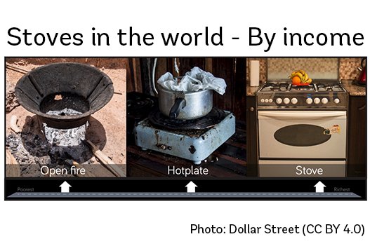
Furthermore, while benchmark datasets, such as ImageNet [@russakovsky2015imagenet], COCO [@lin2014microsoft], Visual Wake Words [@chowdhery2019visual], Google Speech Commands [@warden2018speech], etc. provide a standardized performance metric, they might not capture the diversity and unpredictability of real-world data. Two facial recognition models with similar benchmark scores might exhibit varied competencies when faced with diverse ethnic backgrounds or challenging lighting conditions. Such disparities underscore the importance of robustness and consistency across varied data. For example, Figure 1 from the Dollar Street dataset shows stove images across extreme monthly incomes. So if a model was trained on pictures of stoves found in wealth countries only, it will fail to recognize stoves from poorer regions.

Figure 1: Objects, such as stoves, have different shapes and technological levels in different regions. A model that is not trained on diverse datasets might perform well on a benchmark but fail in real-world applications. Source: Dollar Street stove images.

In essence, a thorough comparative analysis transcends numerical metrics. It’s a holistic assessment, intertwined with real-world applications, costs, and the intricate subtleties that each model brings to the table. This is why it becomes important to have standard benchmarks and metrics that are widely established and adopted by the community.

Formulas

• \(\pi \approx 3.14159\)
• \(\pm \, 0.2\)
• \(\dfrac{0}{1} \neq \infty\)
• \(0 < x < 1\)
• \(0 \leq x \leq 1\)
• \(x \geq 10\)
• \(\forall \, x \in (1,2)\)
• \(\exists \, x \notin [0,1]\)
• \(A \subset B\)
• \(A \subseteq B\)
• \(A \cup B\)
• \(A \cap B\)
• \(X \implies Y\)
• \(X \impliedby Y\)
• \(a \to b\)
• \(a \longrightarrow b\)
• \(a \Rightarrow b\)
• \(a \Longrightarrow b\)
• \(a \propto b\)

\[\color{red}{X \sim Normal \; (\mu,\sigma^2)}\]

Overview

Use the html format to create HTML output. For example:

---
title: "My document"
format:
  html:
    toc: true
    html-math-method: katex
    css: styles.css
---

This example highlights a few of the options available for HTML output. This document covers these and other options in detail. See the HTML format reference for a complete list of all available options.

Table of Contents

Use the toc option to include an automatically generated table of contents in the output document. Use the toc-depth option to specify the number of section levels to include in the table of contents. The default is 3 (which means that level-1, 2, and 3 headings will be listed in the contents). For example:

toc: true
toc-depth: 2

Use the toc-expand option to specify how much of the table of contents to show initially (defaults to 1 with auto-expansion as the user scrolls). Use true to expand all or false to collapse all.

toc: true
toc-expand: 2

You can customize the title used for the table of contents using the toc-title option:

toc-title: Contents

If you want to exclude a heading from the table of contents, add both the .unnumbered and .unlisted classes to it:

### More Options {.unnumbered .unlisted}

The HTML format by default floats the table of contents to the right. You can alternatively position it at the left, or in the body. For example:

format:
  html:
    toc: true
    toc-location: left

The floating table of contents can be used to navigate to sections of the document and also will automatically highlight the appropriate section as the user scrolls. The table of contents is responsive and will become hidden once the viewport becomes too narrow. See an example on the right of this page.

Note that the toc-location option is not available when you disable the standard HTML theme (e.g. if you specify the theme: none or theme: pandoc option).

CSS Styles

To add a CSS stylesheet to your document, just provide the css option. For example:

format:
  html: 
    css: styles.css

Using the css option works well for simple tweaks to document appearance. If you want to do more extensive customization see the documentation on HTML Themes.

LaTeX Equations

By default, LaTeX equations are rendered using MathJax. Use the html-math-method option to choose another method. For example:

format:
  html:
    html-math-method: katex

You can also specify a url for the library to load for a given method:

html-math-method:
  method: mathjax
  url: "https://cdn.jsdelivr.net/npm/mathjax@3/es5/tex-mml-chtml.js"

Available math rendering methods include:

Method	Description
mathjax	Use MathJax to display embedded TeX math in HTML output. The default configuration for MathJax is tex-chtml-full.js which loads all MathJax’s extensions except colorv2 and physics (available using \require{physics}).
katex	Use KaTeX to display embedded TeX math in HTML output.
webtex	Convert TeX formulas to <img> tags that link to an external script that converts formulas to images.
gladtex	Enclose TeX math in <eq> tags in HTML output. The resulting HTML can then be processed by GladTeX to produce images of the typeset formulas and an HTML file with links to these images.
mathml	Convert TeX math to MathML (note that currently only Firefox and Safari natively support MathML)
plain	No special processing (formulas are put inside a span with class="math").

Note that there is more detailed documentation on each of these options in the Pandoc Math Rendering in HTML documentation.

Tabsets

You can use tabsets to present content that will vary in interest depending on the audience. For example, here we provide some example code in a variety of languages:

R

fizz_buzz <- function(fbnums = 1:50) {
  output <- dplyr::case_when(
    fbnums %% 15 == 0 ~ "FizzBuzz",
    fbnums %% 3 == 0 ~ "Fizz",
    fbnums %% 5 == 0 ~ "Buzz",
    TRUE ~ as.character(fbnums)
  )
  print(output)
}

Python

def fizz_buzz(num):
  if num % 15 == 0:
    print("FizzBuzz")
  elif num % 5 == 0:
    print("Buzz")
  elif num % 3 == 0:
    print("Fizz")
  else:
    print(num)

Java

public class FizzBuzz
{
  public static void fizzBuzz(int num)
  {
    if (num % 15 == 0) {
      System.out.println("FizzBuzz");
    } else if (num % 5 == 0) {
      System.out.println("Buzz");
    } else if (num % 3 == 0) {
      System.out.println("Fizz");
    } else {
      System.out.println(num);
    }
  }
}

Julia

function FizzBuzz(num)
  if num % 15 == 0
    println("FizzBuzz")
  elseif num % 5 == 0
    println("Buzz")
  elseif num % 3 == 0
    println("Fizz")
  else
    println(num)
  end
end

Create a tabset via a markdown div with the class name panel-tabset (e.g. ::: {.panel-tabset}). Each top-level heading within the div creates a new tab. For example, here is the markdown used to implement the first two tabs displayed above:

::: {.panel-tabset}
## R

``` {.r}
fizz_buzz <- function(fbnums = 1:50) {
  output <- dplyr::case_when(
    fbnums %% 15 == 0 ~ "FizzBuzz",
    fbnums %% 3 == 0 ~ "Fizz",
    fbnums %% 5 == 0 ~ "Buzz",
    TRUE ~ as.character(fbnums)
  )
  print(output)
}
```

## Python

``` {.python}
def fizz_buzz(num):
  if num % 15 == 0:
    print("FizzBuzz")
  elif num % 5 == 0:
    print("Buzz")
  elif num % 3 == 0:
    print("Fizz")
  else:
    print(num)
```

:::

Tabset Groups

If you have multiple tabsets that include the same tab names, you can define a tabset group. Tabs within a group are all switched together (so in the example above once a reader switches to R or Python in one tabset the others will follow along). For example:

::: {.panel-tabset group="language"}
## R

Tab content

## Python

Tab content
:::

Self Contained

HTML documents typically have a number of external dependencies (e.g. images, CSS style sheets, JavaScript, etc.). By default these dependencies are placed in a _files directory alongside your document. For example, if you render report.qmd to HTML:

Terminal

quarto render report.qmd --to html

Then the following output is produced:

report.html
report_files/

You might alternatively want to create an entirely self-contained HTML document (with images, CSS style sheets, JavaScript, etc. embedded into the HTML file). You can do this by specifying the embed-resources option:

format:
  html:
    embed-resources: true

This will produce a standalone HTML file with no external dependencies, using data: URIs to incorporate the contents of linked scripts, style sheets, images, and videos. The resulting file should be self contained, in the sense that it needs no external files and no net access to be displayed properly by a browser.

Anchor Sections

Hover over a section title to see an anchor link. Enable/disable this behavior with:

format:
  html:
    anchor-sections: true

Anchor links are also automatically added to figures and tables that have a cross reference defined.

Smooth Scrolling

Enable smooth scrolling within the page. By default, smooth scroll is not enabled. Enable/disable it with:

format:
  html:
    smooth-scroll: true

External Links

By default external links (i.e. links that don’t target the current site) receive no special visual adornment or navigation treatment (the current page is navigated). You can use the following options to modify this behavior:

Option	Description
link-external-icon	true to show an icon next to the link to indicate that it’s external (e.g. external).
link-external-newwindow	true to open external links in a new browser window or tab (rather than navigating the current tab).
link-external-filter	A regular expression that can be used to determine whether a link is an internal link. For example ^(?:http:|https:)\/\/www\.quarto\.org\/custom will treat links that start with http://www.quarto.org as internal links (and others will be considered external).

External links are identified either using the site-url (if provided) or using the window.host if no site-url or link-external-filter is provided. For example, here we enable both options and a custom filter:

format:
  html:
    link-external-icon: true
    link-external-newwindow: true
    link-external-filter: '^(?:http:|https:)\/\/www\.quarto\.org\/custom'

You can also specify one or both of these behaviors for an individual link using the .external class and target attribute. For example:

[example](https://example.com){.external target="_blank"}

Reference Popups

If you hover your mouse over the citation and footnote in this sentence you’ll see a popup displaying the reference contents:

   Hover over @xie2015 to see a reference to the definitive book on knitr¹.

This behavior is enabled by default. You can disable it with the following options:

format:
  html:
    citations-hover: false
    footnotes-hover: false

Commenting

This page has commenting with Hypothes.is enabled via the following YAML option:

comments:
  hypothesis: true

You can see the Hypothesis UI at the far right of the page. Rather than true, you can specify any of the available Hypothesis embedding options as a sub-key of hypothesis. For example:

comments:
  hypothesis: 
    theme: clean

You can enable Utterances commenting using the utterances option. Here you need to specify at least the GitHub repo you want to use for storing comments:

comments:
  utterances:
    repo: quarto-dev/quarto-docs

You can also specify the other options documented here.

You may also enable Giscus for commenting using the giscus option. Giscus will store comments in the ‘Discussions’ of a Github repo.

comments:
  giscus: 
    repo: quarto-dev/quarto-docs

Like utterances, you need to specify at least the Git repo you want to use for storing comments. In addition, the repo that you use must:

1. Be public

2. Have the Giscus app installed.

3. Have discussion enabled

Review the Giscus documentation for instructions on setting up Giscus in your repository. Additional options are covered here.

Disabling Comments

If you have comments enabled for an entire website or book, you can selectively disable comments for a single page by specifying comments: false. For example:

title: "Home Page"
comments: false

Includes

For example:

format:
  html:
    include-in-header:
      - text: |
          <script src="https://examples.org/demo.js"></script>
      - file: analytics.html
      - comments.html
    include-before-body: header.html

Minimal HTML

The default Quarto HTML output format includes several features by default, including bootstrap themes, anchor sections, reference popups, tabsets, code block copying, and responsive figures. You can disable all of these built in features at once using the minimal option. For example:

---
title: "My Document"
format:
  html:
    minimal: true
---

When specifying minimal: true you can still selectively re-enable features you do want, for example:

---
title: "My Document"
format:
  html:
    minimal: true
    code-copy: true
---

Footnotes

1. knitr is an R package for creating dynamic documents.